Box–Muller transform
The Box–Muller transform (by George Edward Pelham Box and Mervin Edgar Muller 1958)[1] is a pseudo-random number sampling method for generating pairs of independent, standard, normally distributed (zero expectation, unit variance) random numbers, given a source of uniformly distributed random numbers.
It is commonly expressed in two forms. The basic form as given by Box and Muller takes two samples from the uniform distribution on the interval (0, 1] and maps them to two standard, normally distributed samples. The polar form takes two samples from a different interval, [−1, +1], and maps them to two normally distributed samples without the use of sine or cosine functions.
The Box–Muller transform was developed as a more computationally efficient alternative to the inverse transform sampling method.[2] The Ziggurat algorithm gives an even more efficient method.
Contents |
Basic form
Suppose U1 and U2 are independent random variables that are uniformly distributed in the interval (0, 1]. Let
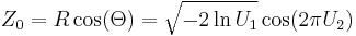
and
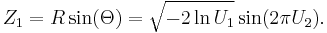
Then Z0 and Z1 are independent random variables with a normal distribution of standard deviation 1.
The derivation[3] is based on the fact that, in a two-dimensional Cartesian system where X and Y coordinates are described by two independent and normally distributed random variables, the random variables for R2 and Θ (shown above) in the corresponding polar coordinates are also independent and can be expressed as
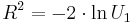
and

Because R2 is the square of the norm of the standard bivariate normal variable (X, Y), it has the chi-squared distribution with two degrees of freedom. In the special case of two degrees of freedom, the chi-squared distribution coincides with the exponential distribution, and the equation for R2 above is a simple way of generating the required exponential variate.
Polar form
The polar form was first proposed by J. Bell[4] and then modified by R. Knop.[5] While several different versions of the polar method have been described, the version of R. Knop will be described here because it is the most widely used, in part due to its inclusion in Numerical Recipes.
Given u and v, independent and uniformly distributed in the closed interval [−1, +1], set s = R2 = u2 + v2. (Clearly  .) If s = 0 or s ≥ 1, throw u and v away and try another pair (u, v). Because u and v are uniformly distributed and because only points within the unit circle have been admitted, the values of s will be uniformly distributed in the open interval (0, 1), too. The latter can be seen by calculating the cumulative distribution function for s in the interval (0, 1). This is the area of a circle with radius
  divided by
  . From this we find the probability density function to have the constant value 1 on the interval (0, 1). Equally so, the angle θ divided by
  is uniformly distributed in the interval [0, 1) and independent of s.
We now identify the value of s with that of U1 and  with that of U2 in the basic form. As shown in the figure, the values of
  and
and  in the basic form can be replaced with the ratios
 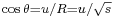 and
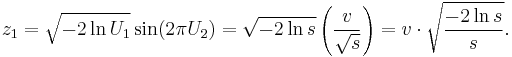
and 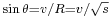 , respectively. The advantage is that calculating the trigonometric functions directly can be avoided. This is helpful when trigonometric functions are more expensive to compute than the single division that replaces each one.
Just as the basic form produces two standard normal deviates, so does this alternate calculation.
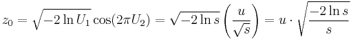
and
Contrasting the two forms
The polar method differs from the basic method in that it is a type of rejection sampling. It throws away some generated random numbers, but it is typically faster than the basic method because it is simpler to compute (provided that the random number generator is relatively fast) and is more numerically robust.[6] It avoids the use of trigonometric functions, which are comparatively expensive in many computing environments. It throws away 1 − π/4 ≈ 21.46% of the total input uniformly distributed random number pairs generated, i.e. throws away 4/π − 1 ≈ 27.32% uniformly distributed random number pairs per Gaussian random number pair generated, requiring 4/π ≈ 1.2732 input random numbers per output random number.
The basic form requires three multiplications, one logarithm, one square root, and one trigonometric function for each normal variate.[7] On some processors, the cosine and sine of the same argument can be calculated in parallel using a single instruction. Notably for Intel-based machines, one can use the fsincos assembler instruction or the expi instruction (usually available from C as an intrinsic function), to calculate complex

and just separate the real and imaginary parts.
The polar form requires two multiplications, one logarithm, one square root, and one division for each normal variate. The effect is to replace one multiplication and one trigonometric function with a single division.
See also
- Inverse transform sampling
- Marsaglia polar method, similar transform to Box-Muller, which uses Cartesian coordinates, instead of polar coordinates
- Ziggurat algorithm, a very different way to generate normal random numbers
References
- ^ G. E. P. Box and Mervin E. Muller, A Note on the Generation of Random Normal Deviates, The Annals of Mathematical Statistics (1958), Vol. 29, No. 2 pp. 610–611
- ^ Kloeden and Platen, Numerical Solutions of Stochastic Differential Equations, pp. 11–12
- ^ Sheldon Ross, A First Course in Probability, (2002), pp. 279–81
- ^ J. Bell: 'Algorithm 334: Normal random deviates', Communications of the ACM, vol. 11, No. 7. 1968
- ^ R. Knopp: 'Remark on algorithm 334 [G5]: normal random deviates', Communications of the ACM, vol. 12, No. 5. 1966
- ^ Everett F. Carter, Jr., The Generation and Application of Random Numbers, Forth Dimensions (1994), Vol. 16, No. 1 & 2.
- ^ Note that the evaluation of 2πU1 is counted as a single multiplication because the value of 2π can be computed in advance and used repeatedly.